Vector Indexing: Wrong Choice Makes Search 100x Slower (2026)
A developer asked why their ChromaDB queries were taking 800ms on a collection of 500,000 vectors. They had never explicitly created an index. ChromaDB had defaulted to HNSW with low ef_construction, which meant the graph was built too sparsely and had to explore far more of the dataset per query to find reasonable neighbors.
Changing hnsw:M from 16 to 32 and hnsw:ef_construction from 100 to 200 at collection creation time — a two-line change — brought latency down to 8ms. But they had to rebuild the collection from scratch because HNSW parameters cannot be changed after the index is built.
Understanding vector indexing is not academic. Index choice and configuration are the primary engineering levers that determine whether your vector search is fast or slow, accurate or approximate, memory-efficient or RAM-hungry.
Concept Overview
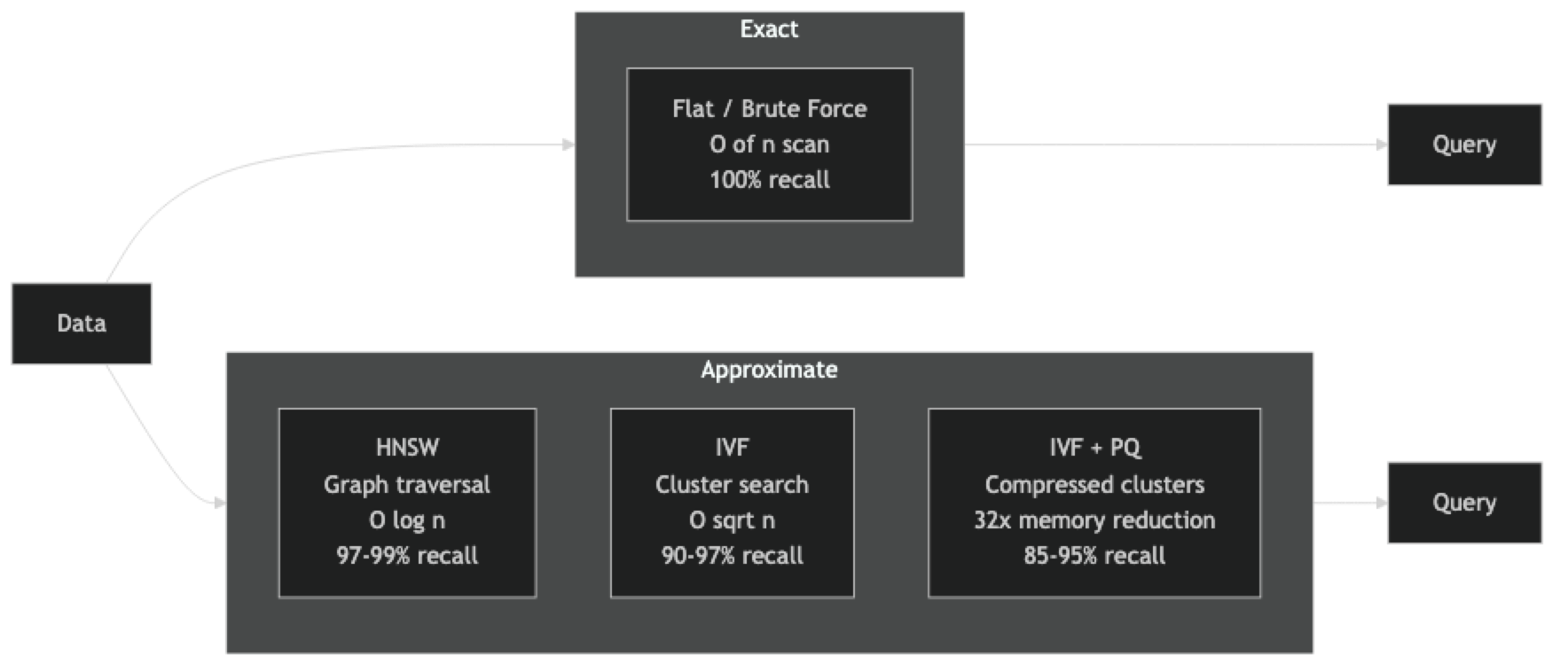
A vector index is a data structure that organizes high-dimensional vectors so that nearest-neighbor queries can be answered faster than O(n) brute-force search.
The design space involves four independent tradeoffs:
Recall vs. latency — exact indexes (flat) give 100% recall but slow queries; approximate indexes (HNSW, IVF) give 95–99% recall at 10–100x lower latency.
Build time vs. query time — HNSW builds slowly (graph construction is expensive) but queries extremely fast. IVF builds faster but requires a training phase. Flat has instant build time.
Memory vs. compression — float32 vectors at 1536 dims take 6KB each. Product quantization compresses to ~200 bytes. The tradeoff is recall quality.
Static vs. dynamic — HNSW supports incremental insertion without rebuilding. IVF degrades in quality when many vectors are added after training. Flat is purely dynamic.
How It Works
Flat index — stores raw vectors in a contiguous array, scans all of them for every query. Zero parameters to tune, zero approximation error. Suitable up to ~100K vectors on CPU, ~10M vectors on GPU.
HNSW — builds a multi-layer graph during insertion. Each node connects to M nearest neighbors in the layer. Top layers have fewer nodes and longer-range connections (for coarse navigation); bottom layers have all nodes and short-range connections (for fine-grained search). At query time, greedy descent through layers finds the approximate nearest neighbors in O(log n).
IVF — trains k-means on a sample to produce C centroid vectors (Voronoi cells). Each vector is assigned to its nearest centroid. At query time, nprobe nearest centroids are identified and only their assigned vectors are scanned. Searching 1% of the dataset gives O(n/100) complexity with reasonable recall.
Product Quantization — splits each vector into M subvectors, quantizes each subvector to one of K codewords using k-means. The final code is M×log2(K) bits. Distance computation uses precomputed lookup tables. Memory reduction is dramatic: a 768-dim float32 vector becomes 48 bytes of codes.
Implementation Example
Flat Index — Baseline for Correctness
import faiss
import numpy as np

DIM = 768
N   = 100_000

np.random.seed(42)
vectors = np.random.randn(N, DIM).astype(np.float32)
faiss.normalize_L2(vectors)   # normalize for cosine similarity

# Flat inner product (= cosine similarity for normalized vectors)
flat = faiss.IndexFlatIP(DIM)
flat.add(vectors)

query = np.random.randn(1, DIM).astype(np.float32)
faiss.normalize_L2(query)

D, I = flat.search(query, k=10)
print(f"Exact top-10 IDs: {I[0]}")
print(f"Exact similarities: {D[0].round(3)}")
HNSW Index — Production Default
import faiss
import numpy as np
import time

DIM = 768
N   = 500_000

vectors = np.random.randn(N, DIM).astype(np.float32)
faiss.normalize_L2(vectors)

# M: connections per node (16=fast build, low mem; 64=slower build, better recall)
# efConstruction: depth of search during graph construction (higher = better graph)
M  = 32
ef = 200

hnsw = faiss.IndexHNSWFlat(DIM, M, faiss.METRIC_INNER_PRODUCT)
hnsw.hnsw.efConstruction = ef

start = time.time()
hnsw.add(vectors)
print(f"HNSW build: {time.time() - start:.1f}s")

hnsw.hnsw.efSearch = 100   # tune at query time — no rebuild needed

query = np.random.randn(1, DIM).astype(np.float32)
faiss.normalize_L2(query)

start = time.time()
D, I = hnsw.search(query, k=10)
print(f"HNSW query: {(time.time() - start)*1000:.2f}ms")
print(f"Top-10 IDs: {I[0]}")

# Memory: ~N * M * 4 bytes for graph + N * DIM * 4 for vectors
graph_mb = N * M * 4 / 1e6
vec_mb   = N * DIM * 4 / 1e6
print(f"Memory: vectors={vec_mb:.0f}MB + graph overhead={graph_mb:.0f}MB")
IVF Index — Scalable Cluster-Based Search
import faiss
import numpy as np
import time

DIM    = 768
N      = 1_000_000
NLIST  = 1000    # number of Voronoi cells; sqrt(N) is a good rule of thumb

vectors = np.random.randn(N, DIM).astype(np.float32)
faiss.normalize_L2(vectors)

quantizer = faiss.IndexFlatIP(DIM)   # used to assign vectors to cells
ivf = faiss.IndexIVFFlat(quantizer, DIM, NLIST, faiss.METRIC_INNER_PRODUCT)

# IVF requires a training phase on a representative sample
train_sample = vectors[:100_000]
print("Training IVF...")
start = time.time()
ivf.train(train_sample)
print(f"Training: {time.time() - start:.1f}s")

ivf.add(vectors)

# nprobe: how many cells to search per query (higher = better recall, slower)
ivf.nprobe = 10   # 10/1000 = 1% of dataset searched

query = np.random.randn(1, DIM).astype(np.float32)
faiss.normalize_L2(query)

D, I = ivf.search(query, k=10)
print(f"nprobe=10  top-10: {I[0]}")

# Tune nprobe for recall tradeoff
for nprobe in [1, 5, 10, 50, 100]:
    ivf.nprobe = nprobe
    start = time.time()
    D, I = ivf.search(query, k=10)
    ms = (time.time() - start) * 1000
    print(f"  nprobe={nprobe:3d}  latency={ms:.2f}ms")
IVF + Product Quantization — Memory-Efficient at Scale
import faiss
import numpy as np

DIM   = 768
N     = 2_000_000
NLIST = 2000   # sqrt(N) ≈ 1414, round up
M_PQ  = 96     # subvectors (DIM must be divisible by M_PQ)
NBITS = 8      # bits per subvector (256 codewords)

vectors = np.random.randn(N, DIM).astype(np.float32)
faiss.normalize_L2(vectors)

quantizer = faiss.IndexFlatIP(DIM)
ivf_pq = faiss.IndexIVFPQ(quantizer, DIM, NLIST, M_PQ, NBITS)

# Requires more training data than IVF alone
ivf_pq.train(vectors[:200_000])
ivf_pq.add(vectors)
ivf_pq.nprobe = 20

query = np.random.randn(1, DIM).astype(np.float32)
faiss.normalize_L2(query)

D, I = ivf_pq.search(query, k=10)

# Memory comparison
float_mb  = N * DIM * 4 / 1e6
pq_mb     = N * M_PQ * NBITS // 8 / 1e6   # M_PQ bytes per vector
print(f"Float32 storage: {float_mb:.0f} MB")
print(f"PQ compressed:   {pq_mb:.0f} MB  ({float_mb/pq_mb:.0f}x reduction)")
ChromaDB HNSW Configuration
import chromadb

client = chromadb.PersistentClient(path="./vector_db")

# HNSW parameters set at collection creation — cannot change later
collection = client.get_or_create_collection(
    name="my_collection",
    metadata={
        "hnsw:space": "cosine",
        "hnsw:M": 32,                # connections per node
        "hnsw:ef_construction": 200, # build quality
        "hnsw:ef_search": 100,       # query quality (can tune per query in some versions)
    },
)

# Add and query
collection.add(
    ids=["v1", "v2", "v3"],
    documents=["HNSW graph indexing", "IVF cluster search", "PQ vector compression"],
)

results = collection.query(query_texts=["approximate nearest neighbor"], n_results=2)
for doc, dist in zip(results["documents"][0], results["distances"][0]):
    print(f"[{1-dist:.3f}] {doc}")
Best Practices
Always establish a flat-index baseline before tuning ANN parameters. The flat index gives you ground truth recall. Running the same queries against flat and your ANN index lets you measure actual recall — not estimated recall from benchmarks on different data.
Size nlist for IVF as sqrt(N) and validate after data grows. If you initially train IVF with 1000 clusters for 1M vectors and later grow to 5M vectors, recall degrades because cells become too large. Rebuild the IVF index when N grows by more than 2–3x.
For HNSW, prefer building with high ef_construction and tuning ef_search at runtime. Index build cost is one-time. Setting ef_construction=200 (vs. the common default of 100) improves graph quality permanently. You can tune ef_search down for latency-critical queries and up for quality-critical queries without rebuilding.
Use IndexHNSWFlat (not IndexHNSWSQ8) for your initial HNSW. Scalar quantization inside HNSW reduces memory but adds approximation error on top of the HNSW approximation. Start with float32 HNSW to isolate recall quality; add scalar quantization later if memory is the binding constraint.
Save and version your indexes with the embedding model version. An index built from text-embedding-3-small version A is incompatible with version B if the model's output vectors change. Treat the index as a deployment artifact tied to the embedding model version.
Common Mistakes
Setting HNSW parameters after adding data. In FAISS's HNSW implementation, you can change efSearch at any time, but M and efConstruction are baked into the graph structure. Building with M=16, then wanting M=32, requires a full rebuild from raw vectors.
Not training IVF on your actual data distribution. IVF's cluster centroids should reflect the geometric structure of your embedding space. Training on random Gaussian samples when your real embeddings cluster around specific topics (e.g., "medical," "legal," "financial") produces imbalanced clusters and poor search quality.
Using IVF for dynamic datasets with many inserts. IVF's cluster assignments are fixed at training time. Vectors inserted after the initial load are assigned to the nearest training centroid, but as more vectors accumulate in specific clusters (because your data shifted), recall degrades. HNSW handles incremental inserts more gracefully.
Forgetting that PQ is lossy at query time, not just at storage time. The distance computed between a float32 query and a PQ-compressed database vector is approximate even if the query vector is exact. This adds another source of approximation error on top of the ANN approximation.
Benchmarking with warm caches only. HNSW query latency is much faster when the entire index fits in the OS page cache. Cold-start latency — the first few queries after loading an index — can be 10–20x higher. Benchmark with cold caches to get realistic production numbers.
Key Takeaways
- HNSW is the production default for most vector databases: it supports incremental inserts, delivers O(log n) query time, and tunable recall at runtime via
ef_search - HNSW parameters
Mandef_constructionare baked into the graph at build time — you cannot change them without rebuilding from scratch - IVF requires a training phase on representative data, degrades with incremental inserts, but uses less memory than HNSW
- Product quantization (PQ) enables billion-scale search by compressing float32 vectors by 8–32x at the cost of additional approximation error
- Always measure recall against a flat-index baseline before declaring your ANN configuration correct
- Size IVF
nlistassqrt(N)and rebuild when data volume grows by more than 2–3x - The decision tree: under 100K vectors use flat; under 50M vectors with RAM use HNSW; over 50M vectors or memory-constrained use IVF or IVF+PQ
- Version your FAISS index files alongside the embedding model version — an index built with one model version is incompatible with another
FAQ
Can I add an HNSW index to existing vectors without rebuilding from scratch? No. HNSW must be built incrementally — each new vector is connected to its nearest existing neighbors during insertion. You cannot "add HNSW" to an already-built flat index. You must start a fresh HNSW index and re-insert all vectors.
What is the memory footprint of an HNSW index?
The graph overhead is approximately N × M × 4 bytes for the connection lists (where M is the parameter you set). For 1M vectors with M=32: 128MB overhead on top of the raw vectors. Total for 1M × 768-dim float32 vectors: ~3GB vectors + 128MB graph = ~3.1GB.
When should I choose IVF over HNSW? When RAM is the binding constraint. IVF does not require storing the entire graph structure in memory — only centroids and the mapping of vectors to clusters. Combined with PQ, IVF allows searching datasets that would not fit in RAM at all for HNSW.
What is scalar quantization in HNSW?
Scalar quantization (SQ) compresses each float32 dimension to int8, reducing vector storage from 4 bytes to 1 byte per dimension (4x compression). IndexHNSWSQ8 in FAISS applies this inside the HNSW index. It gives meaningful memory savings with minimal recall loss compared to PQ, which is more aggressive but less accurate.
How do I choose the M parameter for HNSW? M controls the number of bidirectional connections per node. M=16 is a good default for recall-latency balance with lower memory. M=32 gives better recall at the cost of 2x graph memory overhead. M=64 is used when you need maximum recall and have ample RAM. Start with M=32 for most production workloads.
What nprobe value should I use for IVF? Start with nprobe = sqrt(nlist). For nlist=1000, try nprobe=32 as a baseline. Increase until recall stops improving measurably. Most production systems settle on nprobe = 1–10% of nlist depending on recall requirements. Higher nprobe improves recall linearly but increases latency proportionally.
Can I mix HNSW and IVF in the same system? Yes. Some systems use HNSW for hot recent data (small, fast, in memory) and IVF+PQ for cold historical data (large, compressed, lower recall). A routing layer directs queries to the appropriate index based on data recency or query type.