ANN Algorithms: Pick Wrong and Search Gets 100x Slower (2026)
A team building a product recommendation engine indexed 20 million product embeddings with brute-force cosine similarity. Average query latency: 4.2 seconds. They switched to HNSW. Average query latency: 6 milliseconds. Recall stayed above 99%. The only cost was 3GB of RAM for the index structure.
That 700x speedup is not a coincidence — it is the mathematical consequence of using a graph that exploits the geometry of high-dimensional space rather than scanning every vector. Understanding why ANN algorithms are fast (and when they break down) lets you configure them correctly instead of hoping the defaults work.
Approximate nearest neighbor is the foundational technique that makes vector databases practical. Without it, every vector database would be a slow, O(n) brute-force scan.
Concept Overview
Exact nearest neighbor search in high-dimensional space requires comparing the query against every stored vector — O(n) time complexity that grows linearly with the number of vectors. At 10 million vectors with 1536 dimensions, that is 10 million dot products per query. On a modern CPU, this takes roughly 5 seconds. Completely impractical for interactive use.
ANN algorithms exploit the geometric structure of embedding spaces to find very close neighbors much faster than exact search, trading a small, tunable amount of accuracy for orders-of-magnitude speedup. The tradeoff is controlled: you can always tune toward higher recall at the cost of more compute.
The three dominant ANN algorithm families each make different structural choices:
Graph-based (HNSW) — build a multi-layer proximity graph; search by greedy traversal from a fixed entry point. Excellent recall, low latency, high memory usage.
Inverted File Index (IVF) — partition the vector space into clusters using k-means; at query time, search only the nearest clusters. Lower memory than HNSW, slightly lower recall.
Product Quantization (PQ) — compress vectors into short binary codes; compute approximate distances using lookup tables. Dramatically reduces memory at the cost of recall.
In practice, these are often combined: IVF+PQ (FAISS's IndexIVFPQ) for billion-scale compressed search, HNSW for maximum recall on in-memory datasets.
How It Works
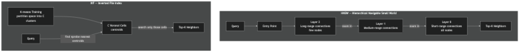
HNSW builds a hierarchy of graphs. The top layer has few nodes connected by long-range links. The bottom layer has all nodes connected to their close neighbors. Search starts at a fixed entry point in the top layer, greedily moves toward the query, then descends to the next layer and repeats. By the time it reaches the bottom layer, it has already narrowed the search to a small local neighborhood. The M parameter controls how many connections each node has; efConstruction controls how thoroughly neighbors are evaluated during construction; efSearch controls how thoroughly the graph is explored at query time.
IVF first trains a k-means clustering on a sample of your vectors, producing C centroids. At index time, each vector is assigned to its nearest centroid. At query time, the algorithm finds the nprobe nearest centroids and searches only the vectors in those clusters. With C=1000 clusters and nprobe=10, you search roughly 1% of the dataset per query.
Implementation Example
HNSW with hnswlib — Fine-Grained Control
pip install hnswlib numpyimport hnswlib
import numpy as np
import time
DIM = 768
N = 100_000
# Build HNSW index
print("Building HNSW index...")
index = hnswlib.Index(space="cosine", dim=DIM)
index.init_index(
max_elements=N,
ef_construction=200, # higher = better quality, slower build
M=32, # connections per node; 16–64 is typical
)
# Generate synthetic data
np.random.seed(42)
vectors = np.random.randn(N, DIM).astype(np.float32)
vectors /= np.linalg.norm(vectors, axis=1, keepdims=True) # normalize
start = time.time()
index.add_items(vectors, ids=np.arange(N))
print(f"Index built in {time.time() - start:.2f}s")
# Query — tune efSearch for recall/latency tradeoff
index.set_ef(100) # higher = better recall, slower query
query = np.random.randn(1, DIM).astype(np.float32)
query /= np.linalg.norm(query)
labels, distances = index.knn_query(query, k=10)
print(f"Top-10 IDs: {labels[0]}")
print(f"Similarities: {1 - distances[0]}") # cosine distance → similarity
# Save and reload
index.save_index("hnsw_index.bin")
index2 = hnswlib.Index(space="cosine", dim=DIM)
index2.load_index("hnsw_index.bin", max_elements=N)FAISS — Multiple Index Types Compared
pip install faiss-cpu numpyimport faiss
import numpy as np
import time
DIM = 768
N = 500_000
QUERY = 100
np.random.seed(42)
vectors = np.random.randn(N, DIM).astype(np.float32)
faiss.normalize_L2(vectors) # normalize for cosine (inner product after normalization)
queries = np.random.randn(QUERY, DIM).astype(np.float32)
faiss.normalize_L2(queries)
def benchmark(index_name: str, index, queries, k: int = 10) -> dict:
start = time.time()
D, I = index.search(queries, k)
elapsed = (time.time() - start) / QUERY * 1000 # ms per query
return {"name": index_name, "latency_ms": elapsed, "results": I}
# --- Flat (exact brute-force, baseline) ---
flat = faiss.IndexFlatIP(DIM) # inner product = cosine for normalized vectors
flat.add(vectors)
r_flat = benchmark("Flat (exact)", flat, queries)
# --- HNSW (approximate, graph-based) ---
hnsw = faiss.IndexHNSWFlat(DIM, 32) # M=32
hnsw.hnsw.efConstruction = 200
hnsw.hnsw.efSearch = 100
hnsw.add(vectors)
r_hnsw = benchmark("HNSW", hnsw, queries)
# --- IVF + Flat (approximate, cluster-based) ---
nlist = 1000 # number of Voronoi cells
quantizer = faiss.IndexFlatIP(DIM)
ivf = faiss.IndexIVFFlat(quantizer, DIM, nlist, faiss.METRIC_INNER_PRODUCT)
ivf.train(vectors) # IVF requires training phase
ivf.add(vectors)
ivf.nprobe = 10 # search 10 of 1000 clusters per query (1%)
r_ivf = benchmark("IVF (nprobe=10)", ivf, queries)
# --- IVF + PQ (compressed, low memory) ---
ivf_pq = faiss.IndexIVFPQ(quantizer, DIM, nlist, 96, 8) # 96 subvectors, 8 bits
ivf_pq.train(vectors)
ivf_pq.add(vectors)
ivf_pq.nprobe = 10
r_ivf_pq = benchmark("IVF+PQ (compressed)", ivf_pq, queries)
# Compare recall for HNSW and IVF vs exact
def recall_at_10(approx_ids, exact_ids):
hits = sum(
len(set(approx_ids[i]) & set(exact_ids[i]))
for i in range(len(exact_ids))
)
return hits / (10 * len(exact_ids))
for r in [r_hnsw, r_ivf, r_ivf_pq]:
recall = recall_at_10(r["results"], r_flat["results"])
print(f"{r['name']:30s} latency: {r['latency_ms']:.2f}ms recall@10: {recall:.3f}")
# Memory usage estimates
print(f"\nMemory (float32 vectors only): {N * DIM * 4 / 1e9:.2f} GB")
print(f"HNSW overhead: ~{N * 32 * 4 / 1e6:.0f} MB for graph connections")
print(f"IVF+PQ storage: ~{N * 96 * 1 / 1e6:.0f} MB for compressed codes")Tuning HNSW Parameters Systematically
import hnswlib
import numpy as np
from itertools import product

def evaluate_hnsw(M: int, ef_construction: int, ef_search: int,
                  vectors: np.ndarray, queries: np.ndarray,
                  exact_ids: np.ndarray, k: int = 10) -> dict:
    dim = vectors.shape[1]
    idx = hnswlib.Index(space="cosine", dim=dim)
    idx.init_index(max_elements=len(vectors), ef_construction=ef_construction, M=M)
    idx.add_items(vectors, ids=np.arange(len(vectors)))
    idx.set_ef(ef_search)

    import time
    start = time.time()
    labels, _ = idx.knn_query(queries, k=k)
    latency = (time.time() - start) / len(queries) * 1000

    recall = sum(
        len(set(labels[i]) & set(exact_ids[i]))
        for i in range(len(queries))
    ) / (k * len(queries))

    return {"M": M, "ef_c": ef_construction, "ef_s": ef_search,
            "latency_ms": latency, "recall": recall}


# Grid search over parameters
N, DIM, Q = 50_000, 384, 200
vecs = np.random.randn(N, DIM).astype(np.float32)
vecs /= np.linalg.norm(vecs, axis=1, keepdims=True)
q = np.random.randn(Q, DIM).astype(np.float32)
q /= np.linalg.norm(q, axis=1, keepdims=True)

# Exact baseline
flat = faiss.IndexFlatIP(DIM)
flat.add(vecs)
_, exact = flat.search(q, 10)

results = []
for M, ef_c, ef_s in product([16, 32], [100, 200], [50, 100, 200]):
    r = evaluate_hnsw(M, ef_c, ef_s, vecs, q, exact)
    results.append(r)
    print(f"M={M:2d} ef_c={ef_c:3d} ef_s={ef_s:3d}  "
          f"latency={r['latency_ms']:.1f}ms  recall={r['recall']:.3f}")
Best Practices
Use HNSW for datasets under 50M vectors where memory is available. HNSW consistently outperforms IVF on recall at the same latency budget. The memory overhead is 20–40% above the raw vector data — acceptable for most use cases.
Use IVF+PQ for billion-scale or memory-constrained deployments. Product quantization compresses 768-dimensional float32 vectors (3072 bytes) to 96 bytes — a 32x reduction with ~10% recall loss at equivalent nprobe. At billion scale, the difference between 3TB and 96GB of RAM is the difference between possible and impossible.
Set ef_construction once based on desired index quality, set ef_search based on latency requirements. A poorly built index (low ef_construction) cannot be fixed by increasing ef_search. Build once with high quality; tune ef_search dynamically for different use cases.
Train IVF on a representative sample of your data, not random vectors. IVF's cluster centroids should reflect the actual distribution of your embeddings. Training on random Gaussian vectors when your real embeddings form topic clusters produces poor partitioning and degraded recall.
Benchmark recall@K, not just query latency. ANN recall degrades silently. Adding many vectors beyond the original max_elements (hnswlib) or beyond the IVF training set size causes recall to drop without any error or warning.
Common Mistakes
Using IndexFlatL2 with text embeddings from OpenAI. OpenAI embeddings are not normalized by default, so euclidean distance and cosine similarity give different rankings. Use IndexFlatIP with manually normalized vectors, or use Chroma/Pinecone which handle this transparently.
Building HNSW with the default M=16 for high-dimensional vectors. The optimal M scales roughly with dimensionality. For 1536-dimensional OpenAI embeddings, M=32 or M=48 gives better recall without proportionally higher memory cost.
Not training IVF on enough vectors. The rule of thumb is 30–100x nlist training vectors. For 1000 clusters, train on 30,000–100,000 vectors minimum. Training on fewer produces imbalanced clusters and poor recall.
Choosing nlist too large for your dataset. The recommended nlist value scales as roughly sqrt(N). For 1 million vectors, use 1000 clusters. For 100,000 vectors, 300 clusters is appropriate. Too many clusters with too few vectors per cluster reduces recall.
Ignoring GPU-accelerated FAISS for batch indexing. If you are building an index over 10+ million vectors, faiss-gpu can build the index 10–50x faster than CPU. This matters when you rebuild indexes regularly — daily or per deployment.
Key Takeaways
- Brute-force vector search is O(n) — at 10 million 1536-dimensional vectors, each query takes roughly 5 seconds on a CPU; ANN algorithms bring this to under 10ms
- HNSW builds a multi-layer graph where the top layers provide long-range shortcuts and the bottom layer contains all nodes — greedy descent achieves O(log n) average complexity
- IVF partitions the vector space into C clusters using k-means and searches only
nprobeclusters at query time — with nprobe=10 out of 1000 clusters, you search just 1% of the dataset per query - Product quantization compresses 768-dimensional float32 vectors (3072 bytes) to 96 bytes — a 32x memory reduction that enables billion-scale search on finite hardware
- HNSW is the right default for most production systems up to 50–100M vectors; IVF+PQ in FAISS or Milvus is the upgrade path for billion-scale or memory-constrained deployments
- Set
ef_constructiononce for index quality — it cannot be recovered after the fact; tuneef_searchdynamically per-query based on latency vs recall requirements - Train IVF on at least 30x the number of clusters — for 1000 clusters train on 30,000 vectors minimum; fewer vectors produces imbalanced clusters and poor recall
- Benchmark recall@K, not just latency — ANN recall degrades silently when dataset size grows beyond the original training distribution
FAQ
What is the recall of HNSW in practice?
With M=32, ef_construction=200, and ef_search=100, HNSW typically achieves 97–99% recall@10 compared to exact brute-force search. You can reach 99.5%+ recall by increasing ef_search to 200–500, at the cost of 2–5x higher latency.
Can I switch from flat (exact) search to HNSW without reindexing? No. HNSW builds a graph during insertion — vectors added to a flat index cannot be converted to HNSW without rebuilding. Plan your index type before loading data.
How does HNSW handle deletions? Most HNSW implementations (including hnswlib and Qdrant) support soft deletes — the vector is marked deleted but the graph connections are not updated. This means deleted vectors still occupy memory and can reduce search quality over time if many deletions accumulate. Periodic index rebuilds are recommended if deletion rate is high.
What is the difference between HNSW and NSW (no hierarchy)? NSW (the original) uses a single flat graph layer. Search complexity is O(log n) on average but degrades to O(n) in worst-case "shortcut-poor" graphs. HNSW adds multiple layers, each with progressively fewer nodes. The top layer provides long-range shortcuts that guarantee O(log n) performance regardless of graph structure.
Is ScaNN better than HNSW? Google's ScaNN achieves better recall at the same latency than HNSW on many benchmarks by using anisotropic quantization tailored to angular distance. However, it is harder to configure, less mature in production tooling, and not integrated into most vector databases. HNSW is the better default; ScaNN is worth evaluating if you need maximum performance on large-scale cloud deployments.
When should I use IVF instead of HNSW? Use IVF+PQ when your dataset exceeds available RAM for HNSW's graph structure or when operating at billion-scale. HNSW requires storing the original vectors plus the graph connections (~40% overhead). IVF+PQ compresses the original vectors dramatically, enabling much larger datasets in the same memory. For datasets under 50M vectors where memory is not constrained, HNSW gives better recall at equivalent latency.
How do I pick nlist for IVF indexing?
The rule of thumb is nlist = sqrt(N) where N is the number of vectors. For 1 million vectors, use 1000 clusters. For 10 million, use 3000–4000. Too few clusters means each cluster is large and nprobe gives you many candidates — slow. Too many clusters with insufficient training data produces imbalanced clusters — poor recall.